Intro

A few years ago, I was curious about implementing a similar approach to the JPEG compression algorithm. I jumped into coding it and found that it was very straight forward, and that the compression rate is (in my opinion) mind-blowing 🤯.

Understanding how it works and, more importantly, what it implies lead me to an audacious idea. This manner of compressing information filters out unnecessary details that humans don’t need to understand the high-level semantics of an image (e.g. knowing that the picture below is of a laptop on a table). Interestingly, the information discarded is also not required for many deep learning tasks, such as some object detection and classification tasks. Therefore, we could potentially use compression to remove “useless” information from an image to facilitate more efficient or faster learning. Let’s explore this idea.

Converting Images to Waves

I’ll keep this brief as there are many high-quality resources available to explain this topic. I’ll also avoid delving into the math and equations.

In an oversimplified sense, JPEG converts an image into a set of sinusoidal functions (sine and cosine functions). Theoretically, you can approximate any function using a linear combination of sine and cosine functions. Images can also be approximated by sine and cosine functions.

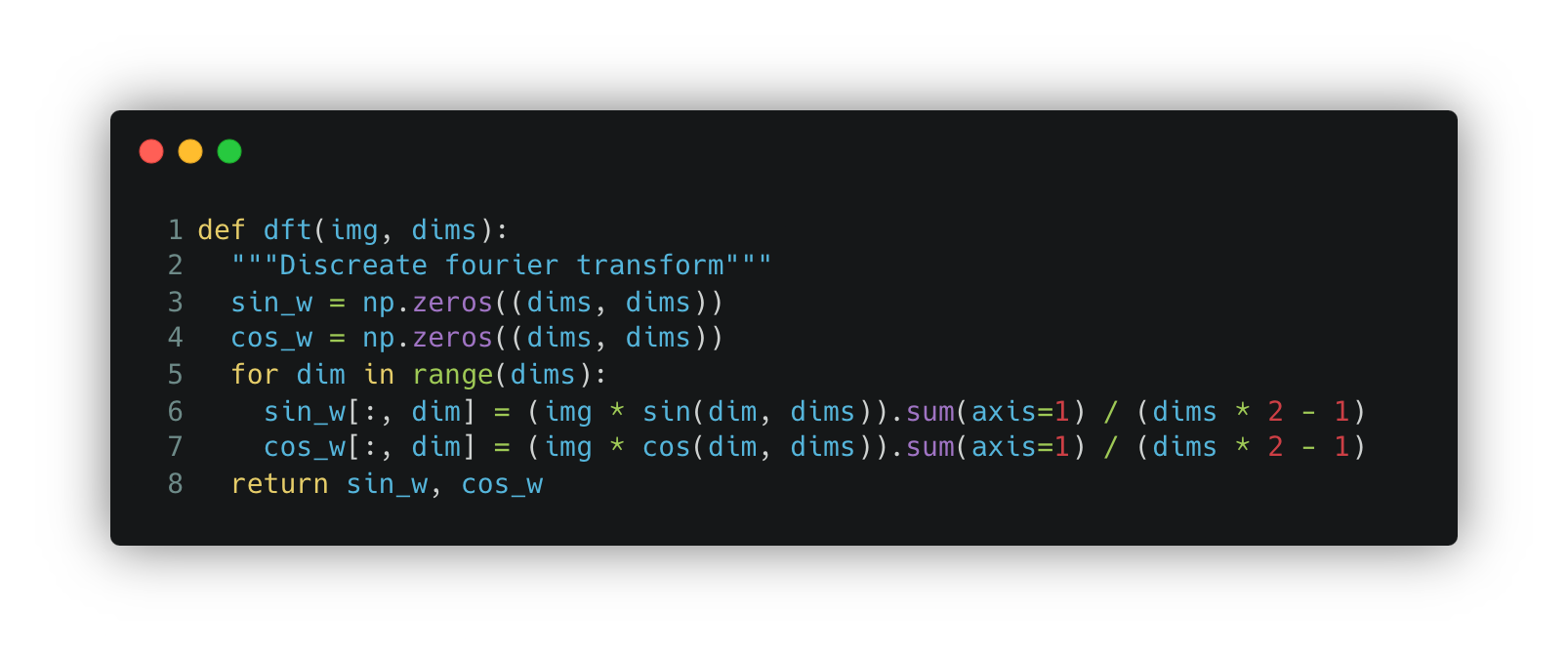
The function that converts an image into a Fourier series is shown below. It converts the image into a sine and cosine of various frequencies and amplitudes. The function returns the weight (or amplitude) of each sine and cosine function. The frequency range is pre-defined by the dimensions of the image. Each sin_w and cos_w forms a matrix the same size as the image, so far we haven’t compressed anything.

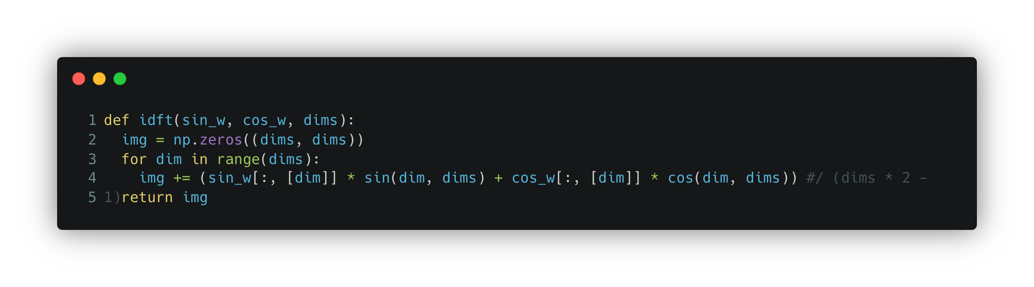
To convert the image back to pixel space from Fourier space, you need to combine all the functions along with their respective weights (a convex linear combination). See the function idft below.

Just to complete this section, I will add the missing functions.

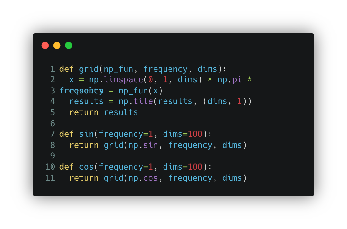
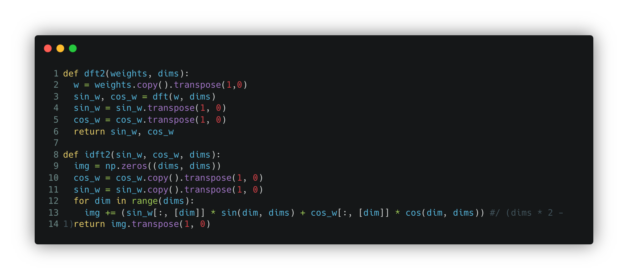
For now, this only includes the transformation for one dimension. You can convert both dimensions into wave signals to capture more patterns.

Compressing Images

What dft returns is the weight that each sine and cosine function has at a specific predefined frequency. A straightforward way to compress is by only saving the functions that contribute significantly to the pixel, i.e., the functions with the largest weights.

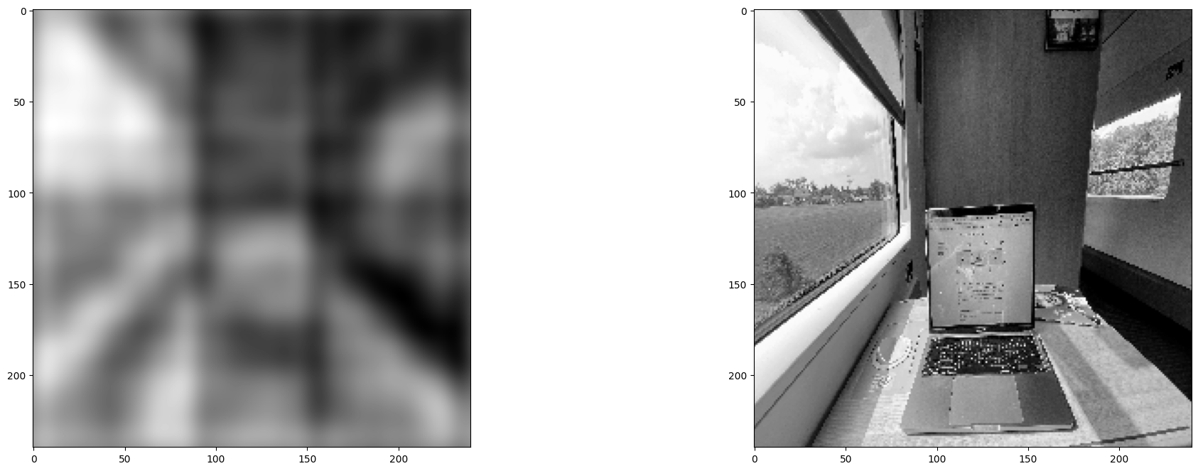
The figure above contains two images. On the right is the original image, and on the left is the compressed image. The left image is using only 1% of the information that the original image uses. You can still perceive some semantics of the image; for example, you can understand that the picture is of a laptop on a table in a room with windows on both sides. However, you are losing some information. For instance, you can no longer distinguish that there is a magazine next to the laptop or that there are trees outside the windows.

The fact that we can compress information a hundredfold while maintaining the high-level information of the picture is extraordinary.

We achieve this level of compression because we retain only those frequencies that contribute the most to the image pixels.

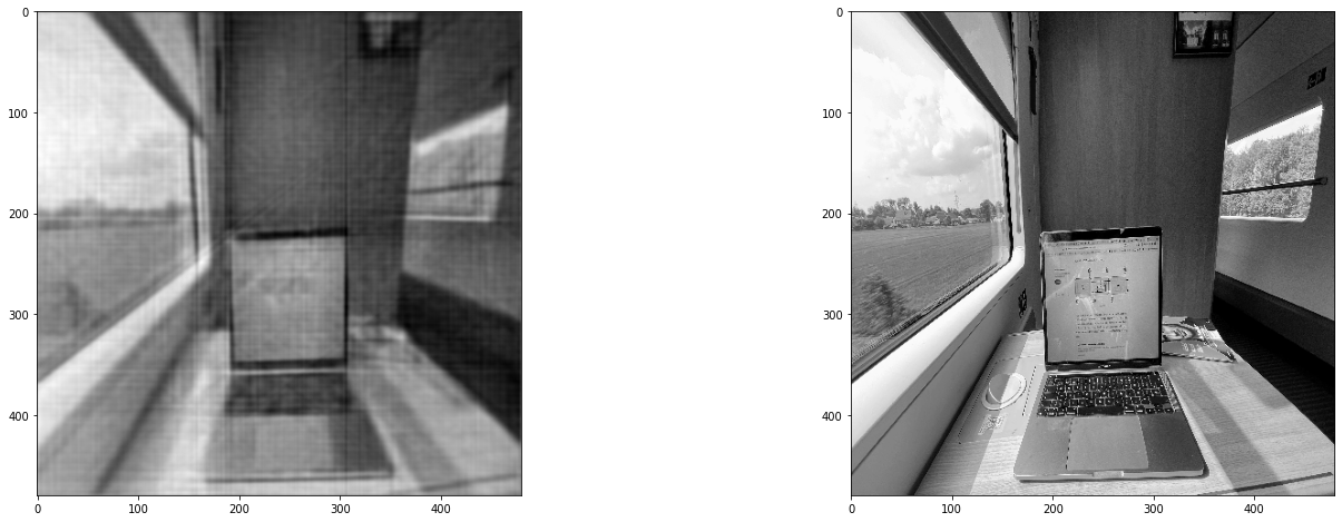
Unfortunately, we can’t continue compressing indefinitely; the image below displays the result of compressing to 0.1% of the original image, unfortunately, it’s too much, and we lose a great deal of the semantics we care about.

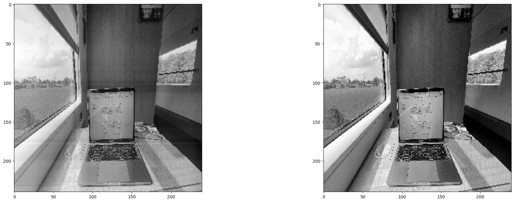
It’s also important to acknowledge that this overly simplified compression is not lossless. Even if we utilize all the full dimensions (i.e., all the weights), we lose some low-level details and introduce some artifacts in the form of horizontal and vertical lines. Depending on the size of the image, we might be losing around 5% of the image (measured using the reconstruction error). The image below shows the reconstructed image using all the information, effectively no compression at all.

Using it in Artificial Neural Networks

This section presents an interesting thought. We mentioned that while compressing the image, we preserve only the heavier frequencies. Coincidentally, on most typical days, all images contain most information in the lowest frequencies. With a naïve implementation, this means that by sharing a fraction (the first dimensions) of the Fourier transformed image, we share most of the high-level semantic information of the image.

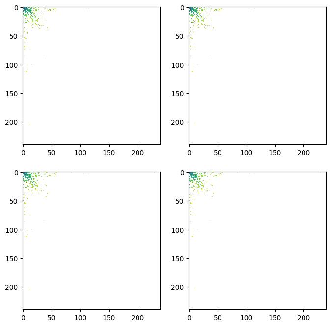
The image above displays the weights of each sinusoidal function. There are four plots because it is a 2D Fourier transform. For your information, the actual values are in logarithmic scale.

What’s more fascinating is that each “pixel” or value of the Fourier transformed image contains more global information. A single value tells us all about that sinusoidal function with the given frequency across the entire image. This means that the neural network can “see” more of the image with a single value. We are effectively making the sharing of information more efficient.

At some point, I believe there was a paper discussing working directly with the jpeg files. I suppose it relates to this idea, but I have yet to try this idea or read that paper. We’ll save that for another day.