A “quick” review of Error State - Extended Kalman Filter
Recently in my job I had to work on implementing a Kalman Filter. My surprise was that there is an incredible lack of resources explaining with detail how Kaman Filter (KF) works. Imagine now the lack of resources explaining a more complex KF as the Error-state Extended Kaman Filter (ES-EKF). In this post, I will focus on the ES-EKF and leave UKF alone for now. One of the only blogs regarding a linear KF worth reading is kalman filter with images which I recommended. Here I will cover with more details the whole linear Kalman filter equations and how to derive them. After that, I will explain how to transform it into an Extended KF (EKF) and then how to transform it into an Error-state Extended KF (ES-EKF).
Notation
We will use Proper Euler angles to note rotations, that will be is \(\alpha, \beta, \gamma\), we are only interested in 2D rotations, therefore, we will use the z-x’-z’’ representation in which \(\alpha\) represents the yaw (the representation does not matter as far as the first rotation happens in the \(z\) axis). The steering angle will be noted by \(\delta\).
Explanation
The Kalman Filter is used to keep track of certain variables and fuse information coming from other sensors such as Inertial Measurement Unit (IMU) or Wheels or any other sensor. It is very common in robotics because it fuses the information according to how certain the measurements are. Therefore we can have several sources of information, some more reliable than others and a KF takes that into account to keep track of the variables we are interested in.
State
The state \(s_t\) we are interested in tracking is composed by \(x\) and \(y\) coordinates, the heading of the vehicle or the yaw \(\theta\), the current velocity \(v\) and steering angle \(\delta\). The tracked orientation is only composed by the yaw \(\theta\), we are only modelling a 2D world, therefore we do not care about the roll \(\beta\) or pitch \(\gamma\). And finally, we added the steering angle \(\delta\) which is important to predict the movement of the car. Therefore the state in timestep \(t\) is
\[s_t= \left[\begin{matrix} x\\y\\\theta\\v\\\delta \end{matrix}\right]\]KF can be divided into two steps, update and predict step. In the predict step, using the tracked information we predict where will the object move in the next step. In the update step, we update the belief we have about the variables using the external measurements coming from the sensors.
Sensor
Keep in mind that a KF can handle any number of sensors, so far we are going to use the localization measurement coming from a GPS + pseudo-gyro.
This measurement contains the global measurements (\(x,y\)) that avoid the system of drifting. This system (without global variables) is also called Dead reckoning. Dead reckoning or using a Kalman Filter without a global measurement is prone to cumulative errors, that means that the state will slowly diverge from the true value.
Prediction Step
We will track the state as a multivariable Gaussian distribution with mean \(\mu\) and covariance \(P\). \(\mu_t\) will be the expected value of the state using the information available (i.e. the mean of \(s_t\)). And the state will have a covariance matrix \(P\) which means how certain we are about our prediction. We will use \(\mu_{t-1}\) and \(u\) to predict \(\mu_t\). Here \(u\) is a control column-vector of any extra information we can use, for example, steering angle if we can have access to the steering of the car or the acceleration if we have access to it. \(u\) can be a vector of any size.
We will try to model everything using matrices but for now, we will use scalars, the new value of the state in \(t\) will be
\[\begin{align} x_t &= x_{t-1} + v\Delta t \cos \theta\\ y_t &= y_{t-1} + v\Delta t \sin \theta\\ \theta &= \theta_{t-1}\\ v_t &= v_{t-1}\\ \delta_t &= \delta_{t-1} \end{align}\]Here we are making simplifying assumptions about the world. First, the velocity \(v\) and the steering \(\delta\) of the next step will be the same as before which is a weak assumption. The strong assumption is that the heading or yaw of the car \(\theta\) is the same. Notice we are not using the steering but we still track it, it will be useful later. We can incorporate the kinematic model here to make the prediction more robust. But that will be adding non-linearities (and so far it is a linear KF). For now, let’s work with a simple environment and later on we can make things more interesting.
This prediction can be re-formulated in matrix form as
\[\mu_t = F\mu_{t-1} + Bu\]Where \(u\) is a zero vector and \(B\) is a linear transformation from \(u\) into the same form of the state \(s\). Also, \(F\) would be (\(F\) has to be linear so far, in the EKF we will expand that to include non-linearities)
\[F = \left[\begin{matrix} 1 & 0 & 0 & \Delta t\cos\theta & 0 \\ 0 & 1 & 0 & \Delta t\sin\theta & 0\\ 0 & 0 & 1 & 0 & 0\\ 0 & 0 & 0 & 1 & 0\\ 0 & 0 & 0 & 0 & 1 \end{matrix}\right]\]This will result in the same equations but using matrix notation. Rember now that we are modelling \(s\) as a multivariable gaussian distribution and we are keeping track of the mean \(\mu\) of the state \(s\) and the covariance \(P\). Using the equations above we update the mean of the state, now we have to update the covariance of the state. Every time we predict we make small errors which add noise and results in a slightly less accurate prediction. The covariance \(P\) has to reflect this reduction in certainty. The way it is done with Gaussian distributions is that the distribution gets slightly more flat (i.e. the covariance “increase”).
In a single-variable gaussian distribution \(y \sim \mathcal N (\mu',\sigma^2)\) the variance has the property that \(\text{var}(ky) = k^2\text{var}(y)\), where \(k\) is a scalar. In matrix notation that is \(P_t = FP_{t-1}F^T\). Now we have to take into account that we are adding \(Bu\), where \(u\) is the control vector and a gaussian variable with covariance \(Q\). The good thing about Gaussians is that the covariances of a sum of Gaussians is the sum of the covariances (if both random variables are independent). Having this into account we have.
\[P_t = FP_{t-1}F^T+BQB^T\]And with this, we have finished prediction the state and updating its covariance.
Update step
In the update step, we receive a measurement \(z\) coming from a sensor. We use the sensor information to correct/update the belief we have about the state. The measurement is a random variable with covariance \(R\). This is where things get interesting. In this case, we have two Gaussians variables, the state best estimate \(\mu_t\) and the measurement reading \(z\).
The best way to combine two Gaussians is by multiplying them together. By multiplying them together, if certain values have high certainty in both distributions, the result will be also a high in the product (very certain). If both values have low certainty, the product will be even lower. And if If only one is high and the other is not, then the result will lay between high and low certainty. So multiplication of Gaussians merges the information of both distributions taking into account how certain the values are (covariance).
The equations derived from multiplying two multivariate Gaussians are similar to the single variable case. We will derive them here and generalize that to matrix form.
Let’s suppose we have \(x_1 \sim \mathcal N (\mu_1,\sigma_1^2)\) and \(x_2\sim\mathcal N(\mu_2,\sigma_2^2)\) (and they do not have anything to do with the state or measurement for now). Have in mind that both \(x_1\) and \(x_2\) live in the same vector space \(x\), therefore
\[\begin{align} p(x_1) = \frac 1 {\sqrt{2\pi\sigma_1^2}}e^{-\frac{(x-\mu_1)^2}{2\sigma_2^2}} & & p(x_2) = \frac 1 {\sqrt{2\pi\sigma_2^2}}e^{-\frac{(x-\mu_2)^2}{2\sigma_2^2}} \end{align}\]by multiplying them together we obtain
\[\frac 1 {\sqrt{2\pi\sigma_1^2}}e^{-\frac{(x-\mu_1)^2}{2\sigma_1^2}}\frac 1 {\sqrt{2\pi\sigma_2^2}}e^{-\frac{(x-\mu_2)^2}{2\sigma_2^2}}\]We also now about a very useful property of Gaussians: the product of Gaussians is also a gaussian distribution. Therefore, to know the result of fusing both Gaussians we have to write the equation above in a gaussian form.
\[\begin{align} &=\frac 1 {\sqrt{2\pi\sigma_1^2}}e^{-\frac{(x-\mu_1)^2}{2\sigma_1^2}}\frac 1 {\sqrt{2\pi\sigma_2^2}}e^{-\frac{(x-\mu_2)^2}{2\sigma_2^2}}\\ &=\frac 1 {2\pi\sigma_1^2\sigma_2^2}e^{-\left(\frac{(x-\mu_1)^2}{2\sigma_1^2}+\frac{(x-\mu_2)^2}{2\sigma_2^2}\right)}\\ \end{align}\]Because we know the result will be a Gaussian distribution, we do not care about constant values (e.g. \(2\pi\sigma_1^2\)), in fact, we only care about the exponent value, which I have to transform it into something similar to
\[\frac{(x-\text{something})^2}{2\text{something else}^2}\]Where \(\text{something}\) will be the new mean and \(\text{something else}^2\) will be the new covariance after multiplication. Therefore we will ignore all the other terms and focus on the exponent value.
\[\begin{align} \frac{(x-\mu_1)^2}{2\sigma_1^2}+\frac{(x-\mu_2)^2}{2\sigma_2^2} &= \frac{\sigma_2^2(x-\mu_1)^2+\sigma_1^2(x-\mu_2)^2}{2\sigma_1^2\sigma_2^2}\\ &= \frac{\sigma_2^2x^2-2\sigma_2^2\mu_1x+\sigma_2^2\mu_1^2 + \sigma_1^2x^2-2\sigma_1^2\mu_2x+\sigma_1^2\mu_2^2}{2\sigma_1^2\sigma_2^2}\\ &= \frac{x^2(\sigma_2^2+\sigma_1^2)-2x(\sigma_2^2\mu_1+\sigma_1^2\mu_2)}{2\sigma_1^2\sigma_2^2}+\frac{\sigma_2^2\mu_1^2+\sigma_1^2\mu_2^2}{2\sigma_1^2\sigma_2^2}\\ &= \frac{(\sigma_2^2+\sigma_1^2)}{2\sigma_1^2\sigma_2^2}\left(x^2-2x\frac{\sigma_2^2\mu_1+\sigma_1^2\mu_2}{\sigma^2+\sigma_2^2}\right)+\frac{\sigma_2^2\mu_1^2+\sigma_1^2\mu_2^2}{2\sigma_1^2\sigma_2^2}\\ \end{align}\]The term on the right can be ignored because it is constant and goes out of the exponent. And the term in parenthesis resembles a perfect square trinomial lacking the last squared term.
\[\begin{align} &= \frac{(\sigma_2^2+\sigma_1^2)}{2\sigma_1^2\sigma_2^2}\left(x^2-2x\frac{\sigma_2^2\mu_1+\sigma_1^2\mu_2}{\sigma^2+\sigma_2^2}\right)\\ &= \frac{(\sigma_2^2+\sigma_1^2)}{2\sigma_1^2\sigma_2^2}\left(x^2-2x\frac{\sigma_2^2\mu_1+\sigma_1^2\mu_2}{\sigma^2+\sigma_2^2} + \left(\frac{\sigma_2^2\mu_1+\sigma_1^2\mu_2}{\sigma^2+\sigma_2^2}\right)^2 - \left(\frac{\sigma_2^2\mu_1+\sigma_1^2\mu_2}{\sigma^2+\sigma_2^2}\right)^2 \right)\\ &= \frac{(\sigma_2^2+\sigma_1^2)}{2\sigma_1^2\sigma_2^2}\left(\left(x-\frac{\sigma_2^2\mu_1+\sigma_1^2\mu_2}{\sigma^2+\sigma_2^2}\right)^2 - \left(\frac{\sigma_2^2\mu_1+\sigma_1^2\mu_2}{\sigma^2+\sigma_2^2}\right)^2 \right)\\ \end{align}\]Ignoring the second term because it is also a constant, the final result of the exponent value is
\[\frac{(\sigma_2^2+\sigma_1^2)}{2\sigma_1^2\sigma_2^2}\left(x-\frac{\sigma_2^2\mu_1+\sigma_1^2\mu_2}{\sigma_1^2+\sigma_2^2}\right)^2 = \frac{\left(x-\frac{\sigma_2^2\mu_1+\sigma_1^2\mu_2}{\sigma_1^2+\sigma_2^2}\right)^2}{\frac{2\sigma_1^2\sigma_2^2}{(\sigma_2^2+\sigma_1^2)}}\]In fact this final form does resemble a Gaussian distribution. The new mean will be what is in the parenhesis with \(x\) and the new covariance will be the denominator divided by 2. To simplify things further along the way, we will re write it like
\[\begin{align} \mu_{\text{new}} &= \frac{\sigma_2^2\mu_1+\sigma_1^2\mu_2}{\sigma_1^2+\sigma_2^2}\\ &= \mu_1 + \frac{\sigma_2^2\mu_1+\sigma_1^2\mu_2}{\sigma_1^2+\sigma_2^2} - \mu_1\\ &= \mu_1 + \frac{\sigma_2^2\mu_1+\sigma_1^2\mu_2-\mu_1(\sigma_1^2+\sigma_2^2)}{\sigma_1^2+\sigma_2^2}\\ &= \mu_1 + \frac{\sigma_2^2\mu_1+\sigma_1^2\mu_2-\mu_1\sigma_1^2-\sigma_2^2\mu_1}{\sigma_1^2+\sigma_2^2}\\ &= \mu_1 + \frac{\sigma_1^2(\mu_2-\mu_1)}{\sigma_1^2+\sigma_2^2}\\ &= \mu_1 + K(\mu_2-\mu_1) \end{align}\]where \(K = \sigma_1^2/(\sigma_1^2+\sigma_2^2)\). For the variance we have
\[\begin{align} \sigma_\text{new}&=\frac{\sigma_1^2\sigma_2^2}{(\sigma_2^2+\sigma_1^2)}\\ &=\sigma_1^2 + \frac{\sigma_1^2\sigma_2^2}{(\sigma_2^2+\sigma_1^2)} - \sigma_1^2\\ &=\sigma_1^2 + \frac{\sigma_1^2\sigma_2^2-\sigma_1^2(\sigma_2^2+\sigma_1^2)}{\sigma_2^2+\sigma_1^2}\\ &=\sigma_1^2 + \frac{\sigma_1^2\sigma_2^2-\sigma_1^2\sigma_2^2+\sigma_1^4}{\sigma_2^2+\sigma_1^2}\\ &=\sigma_1^2 + \frac{\sigma_1^4}{\sigma_2^2+\sigma_1^2}\\ &= \sigma_1^2 + K\sigma_1^2 \end{align}\]Now we need to transform that to matrix notation and change for the correct variables. \(\mu\) and \(z\) are not in the same vector space, therefore to transform \(x\) into the same vector space as the measurement space we use the matrix \(H\). The final result will be
\[\begin{align} K &= HP_{t-1}H^T(HP_{t-1}H^T+R)^{-1}\\ H\mu_t &= H\mu_{t-1}+K(z-H\mu_{t-1})\\ HP_tH^T &= HP_{t-1}H^T+KHP_{t-1}H^T \end{align}\]If we take one \(H\) out from the left of \(K\) and we end up with
\[\begin{align} K &= P_{t-1}H^T(HP_{t-1}H^T+R)^{-1}\\ H\mu_t &= H\mu_{t-1}+HK(z-H\mu_{t-1})\\ HP_tH^T &= HP_{t-1}H^T+HKHP_{t-1}H^T \end{align}\]We can pre-multiply the second and third equation by \(H^{-T}\) and also post-multiply the third equation by \(H^{-1}\), The final result turns out to be in the state vector space \(\mu\) and not in the measurement vector space \(H\mu\). The final result for the update step (which corresponds to the combination of two sources of information with different certainty levels) is
\[\begin{align} K &= P_{t-1}H^T(HP_{t-1}H^T+R)^{-1}\\ \mu_t &= \mu_{t-1}+K(z-H\mu_{t-1})\\ P_t &= P_{t-1}+KHP_{t-1} = (I+KH)P_{t-1} \end{align}\]And that is it! The all the equations for a Linear Kalman Filter.
Prediction step
\[\begin{align} \mu_t &= F\mu_{t-1} + Bu\\ P_t &= FP_{t-1}F^T+BQB^T \end{align}\]Update step:
\[\begin{align} K &= PH^T(HPH^T+R)^{-1}\\ \mu_t &= \mu_{t-1}+K(z-H\mu_{t-1})\\ P_t &= P_{t-1}+KHP_{t-1} = (I+KH)P_{t-1} \end{align}\]Extended Kalman Filter
In reality, the world does not behave linearly. The way KF deals with non-linearities is by using the jacobian to linearize the equation. We can expand this model to a non-linear proper KF modifying the prediction step by adding a simple kinematic model, for example, a bicycle kinematic model.
If we model everything from the centre of gravity of the vehicle, the equations for the bicycle kinematic model are
\[\begin{align} \dot x &= v\cos (\theta+\beta)\\ \dot y &= v\sin(\theta+\beta)\\ \dot \theta &= \frac{v\cos(\beta)\tan(\delta)}{L}\\ \beta &= \tan^{-1}\left(\frac{l_r\tan\delta}{L}\right) \end{align}\]Where \(\theta\) is the heading of the vehicle (yaw), \(\beta\) is the slip angle of the centre of gravity, \(L\) is the length of the vehicle, \(l_r\) is the length between the rearmost part to the centre of gravity and \(\delta\) is the steering angle. In discrete-time form, we will have
\[\begin{align} x_t &= x_{t-1}+\Delta t \cdot v\cos (\theta+\beta)\\ y_t &= y_{t-1}+\Delta t \cdot v\sin(\theta+\beta)\\ \theta_t &= \theta_{t-1} +\Delta t\cdot \frac{v\cos(\beta)\tan(\delta)}{L}\\ \beta_t &= \tan^{-1}\left(\frac{l_r\tan\delta_{t-1}}{L}\right)\\ v_t &= v_{t-1}\\ \delta_t &= \delta_{t-1} \end{align}\]If you define that system of equations as \(\mathbf f(x,y,\theta,v,\delta)\in\mathbb R^6\) then we can model the whole system using \(\mathbf f\) and \(F=\partial f_j/\partial x_i\). We can also use the same trick with the transformation from state space \(s\) into measurement vector space \(z\).
We can also add non-linearities in the measurement. Before we used the matrix \(H\) now we can use the function \(\mathbf h(\cdot)\) and define \(H\) as \(H=\partial h_i/\partial x_i\). The final Extended Kalman Filter is
Prediction step
\[\begin{align} \mu_t &= \mathbf f(\mu_{t-1}) + Bu\\ P_t &= FP_{t-1}F^T+BQB^T\\ \end{align}\]Update step:
\[\begin{align}K &= P_{t-1}H^T(HP_{t-1}H^T+R)^{-1}\\ \mu_t &= \mu_{t-1}+K(z-\mathbf h(\mu_{t-1})) \\P_t &= (I+KH)P_{t-1} \end{align}\]##
Error state - Extended Kalman Filter
EKF is not a perfect method to estimate and predict the state, it will always make mistakes when predicting. The longer the number of sequential predictions without updates, the bigger the accumulated error. One interesting common property of the errors is that they have less complex behaviour than the state itself. This can be seen easier in the image below. While the behaviour of the position is highly non-linear, the error (estimation - ground truth) behaves much closer to a linear behaviour.
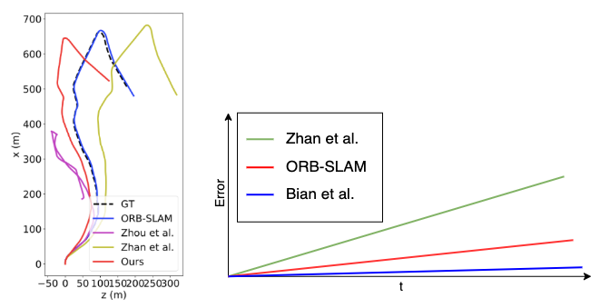
left image taken from “Unsupervised Scale-consistent Depth and Ego-motion Learning from Monocular Video”.
Therefore modelling the error of the state (i.e. error-state) is more likely that will be model correctly by a linear model. Therefore, we can avoid some noise coming from trying to model highly non-linear behaviour by modelling the error-state. Let’s define the error-state as \(e=\mu_t-\mu_{t-1}\). We can approximate \(\mathbf f(\mu_{t-1})\) using the Taylor series expansion only using the first derivative. Therefore \(\mathbf f(\mu_{t-1}) \approx \mu_{t-1} + Fe_{t-1}\). Replacing this and rearranging equation we end up with the final equations for the Error state - Extended Kalman Filter (ES-EKF)
Prediction step
\[\begin{align} s_t &= \mathbf f(s_{t-1},u)\\ P_t &= FP_{t-1}F^T+BQB^T\\ \end{align}\]Update step:
\[\begin{align}K &= PH^T(HPH^T+R)^{-1}\\ e_t &= K(z-h(\mu_{t-1}))\\ s_t &= s_{t-1} + e_t\\ P_t &= (I+KH)P_{t-1} \end{align}\]Keep in mind that now we are tracking the error state and the covariance of the error, therefore we need to predict the state \(s_t\) and correct it by using the error-state during the update step, otherwise, we can estimate the state directly using \(\mathbf f(\cdot)\) as in ithe prediction step.
(if you see I have made a mistake, don’t hesitate to tell me).