Unsupervised Depth Estimation Explained 1
Lately, there have been several interesting papers 2345678910111213141516 for depth estimation using only images and without any supervision. Some approaches use stereo images, some others use scale consistency to improve results, there are implementations with multiple masks as well as a very simple defined mask to filter out moving objects or occluded or new visible objects.
Repository
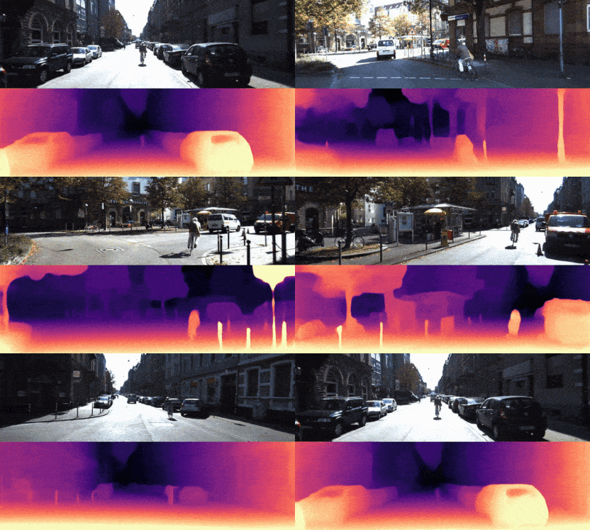
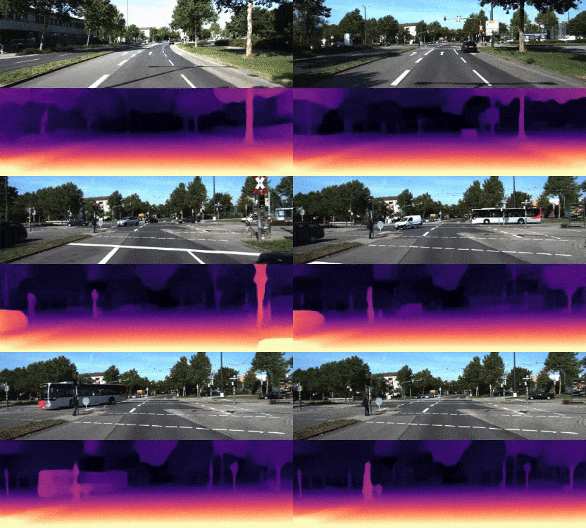
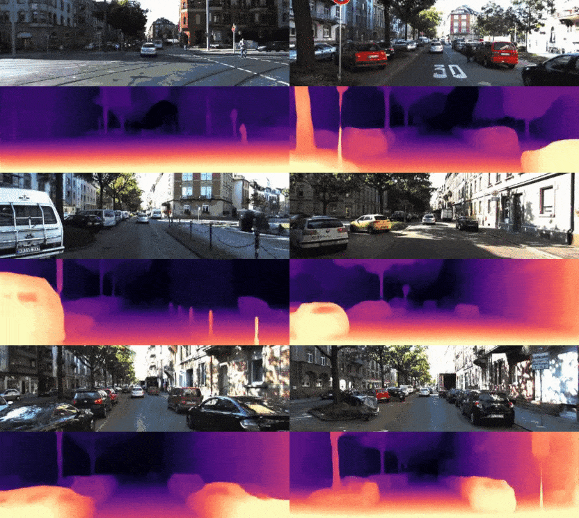
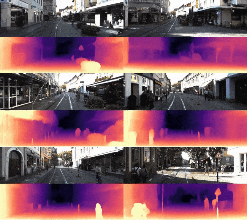
A basic implementation of this idea available here, and an extension of monodepth2 is available here. Here are some results of the extended monodepth2 model:
 |
 |
|---|---|
 |
 |
Explanation
If I am not mistaken, the first paper using this unsupervised approach with deep NN was Godard et al. 8 using epipolar geometry to infer depth. They built on top of Garg et al. 5 which used similar methods but the transformation matrix was given. I will mainly discuss the approach of Zhou et al. 2, because it is a good foundation for the rest of the papers.
All the models cited here are based on the general equation of 3D to 2D image projection equation:
\[\begin{equation} z_c \begin{bmatrix}u\\v\\1\end{bmatrix} = K[R|\boldsymbol t]\begin{bmatrix}x_w\\y_w\\z_w\\1\end{bmatrix} \end{equation}\]This equation coverts a 3D homogenous world coordinate \([x_w,y_w,z_w,1]^T\) into pixel homogeneous coordinate \([u,v,1]^T\), here \(K\) is know as the intrinsic matrix and holds all the intrinsic parameters of the camera, such as focal length \(f\), the principal point (which is the centre of the image in pixels) but does not include the distortion parameters. All modern cameras have a certain degree of distortion produced by its lens, it is the same distortion produced by a fisheye lens but with a varying degree. The projection equation we saw above (a.k.a. pinhole camera model) does not include any term accounting for this kind of distortions. For this equation we assume there is no lens, therefore the distortion correction has to happen before using this model, this is usually done by the camera itself.
\([R\mid \boldsymbol t]\) represents the transformation matrix, \(R\) stands for Rotation and \(t\) for translation, there are several different ways of representing rotation and translation of a body in 3D space, the easiest to use is the 6 degrees of freedom, which is used by all the papers here. We use Euler angles to represent rotations, but there are also quaternions and rotation matrices. 6 DoF has 6 variables, three for the translation in \(x,y\) and \(z\) axis and three for the rotation (Euler angles) in each corresponding axis (roll, pitch and yaw respectively).
To transform/rotate an object, it is necessary to convert the 6DoF into the transformation matrix, there are several interesting materials out there regarding how to do it. The result of that operation is the following matrix
\[[R|\boldsymbol t] = \begin{bmatrix}R&\boldsymbol t\\\boldsymbol 0 &1\end{bmatrix}\]Where \(R\) is the rotation matrix (have in mind that \(R\) is not the same as the Euler angles but comes from them) and \(\boldsymbol t\) is the translation in the 3D world \([t_x,t_y,t_z]^T\).
Finally, \(z_c\) is the depth from the camera frame and can be considered the scaling factor. The subscript \(c\) means it is in respect to the camera frame, where for instance \(w\) would mean it is in the world coordinates.
Usually, the models cited, use a target and a source image. Some use two sources to improve the results, nonetheless, the concept is the same. The target is the image being predicted and the source is the image used to predict the target. The main equation of Zhou et al. 2 follows the following logic. The first step is to covert the coordinates of the target image (\(x\)-\(y\) pixels, a normal mesh grid) into world coordinates, by doing this
\[K^{-1}I_{grid} \cdot {z_{\text{w}}^\text{target}} \leftarrow \text{This is in world coordinates}\]\(I_\text{grid}\) are all the coordinates of the pixels. This operation is exactly the opposite showed above, instead of projecting 3D world points into an image, this converts 2D images into a cloud point. Because going from 3D to 2D we drop information (mainly the depth), going from 2D to 3D need extra information to reconstruct the 3D point cloud, we add this lost information (depth) when multiplying by \(z_w^\text{target}\). If you solve for the 3D world coordinates in the first equation, this is the same operation with no translation nor rotation.
Next, this result is translated again, from the target location to the source location using the camera movement \([K\mid\boldsymbol t]_{\text{target}\to\text{source}}\). Then it is converted again into pixel coordinates by multiplying the result by the intrinsic matrix \(K\).
\[I_\text{source_coords} \leftarrow \underbrace{K[R|\boldsymbol t]_{\text{target}\to\text{source}}}_{\texttt{proj_tgt_cam_to_src_pixel}}\underbrace{\left( K^{-1}I_{grid}* {z_{\text{camera}}^\text{target}} \right)}_{\texttt{cam_coords}}\]With this, we have “matched” the coordinates from the target image with coordinates from the source image. In other words, we know where each pixel in the target image should go in the source image. That means that we can reconstruct the target image from pixels from the source image. The common way of doing this is using bilinear interpolation, which could be considered as a “convex” combination of the pixels’ colours where the weights are the distance between the pixels coordinates.
\[I_\text{projected_target} = B(I_\text{source_coords},I_\text{source})\]This is called inverse warp because instead of sending the pixels from source to target, it matches the pixels from target to source and from there reconstruct the target. If I am not mistaken (if I am, correct me) in this way the projection into target pixels does not have fractional pixels (e.g. \((3.3,2.5)\)) and the bilinear interpolation is done in the source image.
This reconstruction will have several dead pixels. Not even in a perfect world, this matching operation could be a bijection between the two frames. For example pixels of the scene that were not visible in the source but were visible in the target will not have a match in the other image. Apart from these dead pixels, objects moving (dynamic objects) will have a different position in the next frame. For them, estimating depth from the target is not enough, they will also require estimating their motion. All those impossible to match pixels are also predicted and the list of pixels that are not predictable are put in a Mask \(M\). If \(M\) is all the non-predictable pixels (due to occlusion, dynamic objects, etc.) then \(1-M\) is all the predictable pixels. There are different ways of predicting these un-matchable pixels, for an interesting approach see Bian et al. 14
From there, basically the loss is the reconstruction loss between the predictable pixels between the projected image and the target image. That is:
\[\mathcal L = \sum_\text{pixels}|I_\text{projected_target}-I_\text{target}|(1-M)\]For this, it was necessary to estimate the depth of the target \(z_\text{camera}^\text{target}\) and the movement of the camera (ego-motion) \([R\mid\boldsymbol t]\). That is the basic approach, there we were given the intrinsic matrix, one extra step is to estimate the intrinsic matrix \(K\) as well, which several approaches do. It is also possible to differentiate between unpredictable pixels and dynamic objects and try to predict its movement.
Finally, it is important to mention that the entire loss function includes terms for smoothness as well as regularisation terms, which I don’t cover here because the focus is depth estimation.
(if you see I have made a mistake, don’t hesitate to tell me).
-
Zhou, T., Brown, M., Snavely, N., & Lowe, D. G. (2017). Unsupervised Learning of Depth and Ego-Motion from Video. 2017 IEEE Conference on Computer Vision and Pattern Recognition (CVPR), 6612–6619. https://doi.org/10.1109/CVPR.2017.700 ↩ ↩2 ↩3 ↩4
-
Gordon, A., Li, H., Jonschkowski, R., & Angelova, A. (2019). Depth from Videos in the Wild: Unsupervised Monocular Depth Learning from Unknown Cameras. ArXiv Preprint ArXiv:1904.04998. ↩
-
Mahjourian, R., Wicke, M., & Angelova, A. (2018). Unsupervised learning of depth and ego-motion from monocular video using 3d geometric constraints. Proceedings of the IEEE Conference on Computer Vision and Pattern Recognition, 5667–5675. ↩
-
Garg, R., BG, V. K., Carneiro, G., & Reid, I. (2016). Unsupervised cnn for single view depth estimation: Geometry to the rescue. European Conference on Computer Vision, 740–756. ↩ ↩2
-
Wang, C., Miguel Buenaposada, J., Zhu, R., & Lucey, S. (2018). Learning depth from monocular videos using direct methods. Proceedings of the IEEE Conference on Computer Vision and Pattern Recognition, 2022–2030. Retrieved from https://arxiv.org/abs/1712.00175 ↩
-
Pillai, S., Ambru\cs, R., & Gaidon, A. (2019). Superdepth: Self-supervised, super-resolved monocular depth estimation. 2019 International Conference on Robotics and Automation (ICRA), 9250–9256. Retrieved from https://arxiv.org/abs/1810.01849 ↩
-
Godard, C., Mac Aodha, O., & Brostow, G. J. (2016). Unsupervised Monocular Depth Estimation with Left-Right Consistency. CoRR, abs/1609.0. Retrieved from http://arxiv.org/abs/1609.03677 ↩ ↩2
-
Ranjan, A., Jampani, V., Balles, L., Kim, K., Sun, D., Wulff, J., & Black, M. J. (2019). Competitive Collaboration: Joint Unsupervised Learning of Depth, Camera Motion, Optical Flow and Motion Segmentation. Proceedings of the IEEE Conference on Computer Vision and Pattern Recognition, 12240–12249. Retrieved from https://arxiv.org/abs/1805.09806 ↩
-
Yin, Z., & Shi, J. (2018). Geonet: Unsupervised learning of dense depth, optical flow and camera pose. Proceedings of the IEEE Conference on Computer Vision and Pattern Recognition, 1983–1992. Retrieved from https://arxiv.org/abs/1803.02276 ↩
-
Zhan, H., Garg, R., Saroj Weerasekera, C., Li, K., Agarwal, H., & Reid, I. (2018). Unsupervised learning of monocular depth estimation and visual odometry with deep feature reconstruction. Proceedings of the IEEE Conference on Computer Vision and Pattern Recognition, 340–349. Retrieved from https://arxiv.org/abs/1803.03893v3 ↩
-
Godard, C., Mac Aodha, O., & Brostow, G. J. (2018). Digging Into Self-Supervised Monocular Depth Estimation. CoRR, abs/1806.0. Retrieved from http://arxiv.org/abs/1806.01260 ↩
-
Zhou, T., Brown, M., Snavely, N., & Lowe, D. G. (2017). Unsupervised Learning of Depth and Ego-Motion from Video. 2017 IEEE Conference on Computer Vision and Pattern Recognition (CVPR), 6612–6619. https://doi.org/10.1109/CVPR.2017.700 ↩
-
Bian, J.-W., Li, Z., Wang, N., Zhan, H., Shen, C., Cheng, M.-M., & Reid, I. (2019). Unsupervised Scale-consistent Depth and Ego-motion Learning from Monocular Video. ArXiv Preprint ArXiv:1908.10553. ↩ ↩2
-
Zou, Y., Luo, Z., & Huang, J.-B. (2018). Df-net: Unsupervised joint learning of depth and flow using cross-task consistency. Proceedings of the European Conference on Computer Vision (ECCV), 36–53. Retrieved from https://arxiv.org/abs/1809.01649 ↩
-
Li, Z., Dekel, T., Cole, F., Tucker, R., Snavely, N., Liu, C., & Freeman, W. T. (2019). Learning the Depths of Moving People by Watching Frozen People. Retrieved from http://arxiv.org/abs/1904.11111 ↩